Thermal Systems

This week we simulated a thermal system using matlab, specifically a cup of hot coffee.

1. Simulation of a cooling cup of coffee
We found that when we varied parameters Rth and C:
Higher Rth and C= smaller dT and thterefore the less the temperature will change
Lower Rth and C =larger dT and therefore the more the temperature will change

Original Coffee Plot R=.85 C=10,000

Coffee Plot Rth=10

Coffee Plot Rth=.15

Coffee Plot C=50

Coffee Plot C=1,000,000

2. Let's add a heater
We found that if we want our coffee to heat up to the Starbucks ideal 84 degrees C
This was calculated by using the equation (shown below) and isolation the value P with

T=375 because that's what we want the coffee temperature to be (the heater temperature)

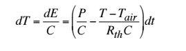
We then incorporated the heater into the program to see hoe the heater effected the program and we could deduce that: 

Rth is the change in final temperature divided by P, which means that final temperature difference depends only on P and Rth. And at equilibrium energy into the system is balanced by energy out.

C is equal to P times dT/dt so at t=0 the slope of the graph is equal to P/C

3. Feedback and Control: Bang Bang

Bang Bang control is appropriate for many thermal systems because it either turns on or off which is good because we only need it to do one thing set the temperature in the room equal to the value inputted, but it is insufficient because if the temperature goes over the right temperature it will have to keep turning itself on and off to again reach the goal temperature.

A zoomed in picture of the plot

4. Proportional Control

Compared to Bang Bang, Proportional control takes a far longer time to reach the desired temperature, this is due to the very nature of proportional control which "slows down" once it gets close to the goal. These models makes sense because in real life thermometers use bang bang control instead of proportional control, and when we compare the graphs it takes ~800 seconds for Bang Bang and ~3000 seconds for Proportional.

5. Add delay:

In reality are are tons of delays because nothing is instantaneous, so we modeled the delay between the time the coffee reaches a given temperature and when the temperature sensor records the 

temperature.

Proportional Control:

The impact of the sensor delay for proportional is that there are no temperature measurements for the first ~450 seconds and then there is a huge jump that then goes back down to a more stable (but still slightly fluctuating) temperature.

Added delay for Bang Bang:
The impact of the sensor delay is that the graph is shifted to the right. This makes sense because bang bang is just "on or off" so the delay in sensing should not change the shape of the graph.

Other delays that we should consider in a thermodynamic system is the time it takes for the heater itself to heat up.

MATLAB Introduction

 Matlab is a computing program that is widely used by engineers for modeling. Or as Allen Downey likes to call it: "a glorified calculator.
First exercise:
Exercise 1   The Fibonacci sequence, denoted F, is described by the equations F₁ = 1, F₂ = 1, and for i ≥ 3, F_i = F_i−1 + F_i−2. The elements of this sequence occur naturally in many plants, particularly those with petals or scales arranged in the form of a logarithmic spiral.
The following expression computes the nth Fibonacci number:

			(1)

We accomplished this task by putting the equation into matlab and checking it by plugging numbers into the program.

Exercise 2
Imagine that you are the owner of a car rental company with two locations, Albany and Boston. Some of your customers do “one-way rentals,” picking up a car in Albany and returning it in Boston, or the other way around. Over time, you have observed that each week 5% of the cars in Albany are dropped off in Boston, and 3% of the cars in Boston get dropped off in Albany. At the beginning of the year, there are 150 cars at each location.

Write a script called car_update that updates the number of cars in each location from one week to the next. The precondition is that the variables a and b contain the number of cars in each location at the beginning of the week. The postcondition is that a and b have been modified to reflect the number of cars that moved.

Our first inclination was to use an exponential function, which in theory works but in practice we realized that it did not update, so we made it instead to have:
anew = a - 0.05*a + 0.03*b; % albany cars after certain number of weeks

bnew = b + 0.05*a - 0.03*b; % boston cars after certain number of weeks

Exercise 3
Create a script named car_loop that uses a for loop to run car_update 52 times. Remember that before you run car_update, you have to assign values to a and b. For this exercise, start with the values a = 150 and b = 150.
If everything goes smoothly, your script will display a long stream of numbers on the screen. But it is probably too long to fit, and even if it fit, it would be hard to interpret. A graph would be much better!

Exercise 4
Modify car_loop so that each time through the loop it plots the value of aversus the value of i.
Once you get that working, modify it so it plots the values of a with red circles and the values of b with blue diamonds.

Exercise 5
We have already seen the Fibonacci sequence, F, which is defined recurrently as

Fi = Fi−1 + Fi−2

In order to get started, you have to specify the first two elements, but once you have those, you can compute the rest. The most common Fibonacci sequence starts with F₁ = 1 and F₂= 1.

Write a script called fibonacci2 that uses a for loop to compute the first 10 elements of this Fibonacci sequence. As a postcondition, your script should assign the 10th element to ans.

Now generalize your script so that it computes the nth element for any value of n, with the precondition that you have to set n before you run the script. To keep things simple for now, you can assume that n is greater than 0.

Exercise 6
The ratio of consecutive Fibonacci numbers, F_n+1/F_n, converges to a constant value as nincreases. Write a script that computes a vector with the first n elements of a Fibonacci sequence (assuming that the variable n is defined), and then computes a new vector that contains the ratios of consecutive Fibonacci numbers. Plot this vector to see if it seems to converge. What value does it converge on?